
The mathematical relationship between variables such as cholesterol levels and blood pressure is a cornerstone of clinical diagnostics, yet the reliability of these correlations is frequently undermined by a fundamental misunderstanding of sample size. When a correlation of 0.62 is observed in a study of 10 patients, researchers often face a critical dilemma: is this a genuine biological signal or merely a statistical artifact? While high-dimensional studies—such as those measuring 20,000 gene expression levels in a handful of mice—routinely apply stringent multiple-testing corrections, smaller studies often operate under the dangerous assumption that they are less susceptible to spurious results. However, recent geometric and statistical analyses reveal that the distribution of a sample correlation is independent of the number of variables measured and depends almost entirely on the number of subjects involved. High-dimensional datasets do not inherently create spurious correlations; they simply provide a larger field of play in which these inevitable artifacts are easier to encounter.

The Mathematical Framework of Correlation Geometry
To understand why spurious correlations occur, one must look beyond the numerical output of a statistical software package and examine the underlying geometry of Pearson’s correlation coefficient ($r$). The process of calculating a correlation involves several transformative steps that project raw data onto a specific mathematical manifold. When we measure $d$ variables across $n$ individuals, we are essentially working with vectors in an $n$-dimensional space.

The first step in calculating Pearson’s $r$ is centering the data. This involves subtracting the sample mean from each observation within a column. Geometrically, this operation shifts the data vectors so that they lie within an $(n-1)$-dimensional subspace that is perpendicular to the vector of ones. For a sample size of $n=3$, this centering constrains all possible data vectors to a two-dimensional plane within a three-dimensional coordinate system. For $n=4$, the vectors are restricted to a three-dimensional hyperplane. This reduction in dimensionality is a fundamental property of the centering process, effectively removing the "location" information from the dataset and focusing solely on the variance.

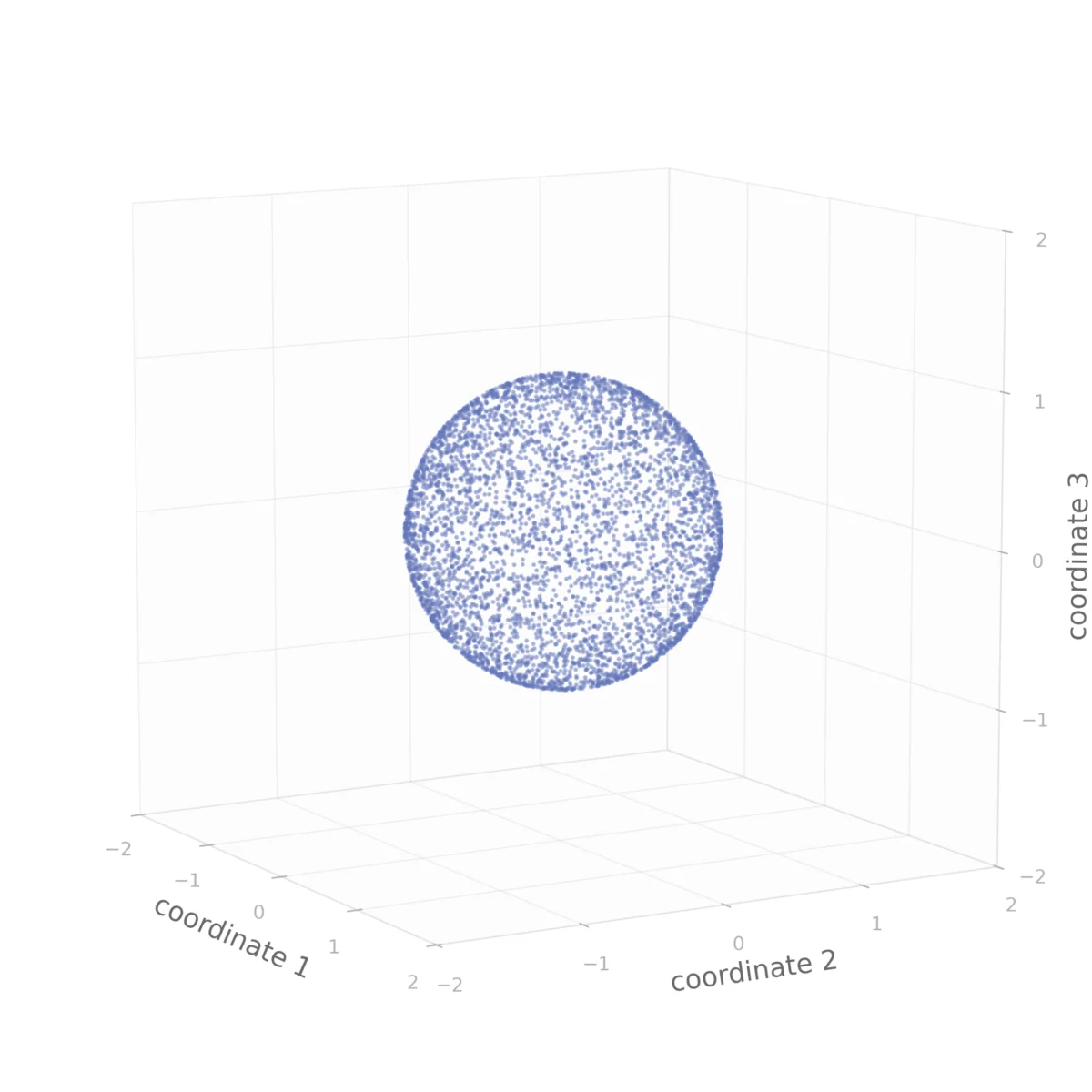
The second step is normalization, where the centered vectors are divided by their magnitude (standard deviation). This moves the vectors onto a unit sphere. In a study with $n=3$, where vectors were already constrained to a plane, normalization forces them onto a one-dimensional unit circle. For $n=4$, the vectors are placed on the surface of a three-dimensional unit sphere. At this stage, the correlation between two variables is redefined as the cosine of the angle between these two normalized vectors. Consequently, the distribution of sample correlations between independent variables is identical to the distribution of the cosines of angles between random points on an $(n-2)$-dimensional manifold.

The Gaussian Experiment: How Chance Mimics Design
In a controlled simulation where variables are drawn from independent Gaussian (normal) distributions, the population correlation is exactly zero. However, the observed sample correlation is almost never zero. Because the standard multivariate normal distribution is rotationally invariant—meaning its density depends only on distance from the origin rather than direction—the vectors, once normalized, become uniformly distributed across the unit sphere.

This rotational invariance allows mathematicians to derive the exact sampling distribution of the correlation $C$. The probability density function of these correlations is governed by the Beta function, where the variance decreases at a rate of $1/(n-1)$. This implies that the typical magnitude of a correlation observed purely by chance is proportional to the inverse square root of the sample size.

The behavior of this distribution at very small sample sizes is particularly counterintuitive:

- For n = 3: The distribution is U-shaped, resembling a rescaled arcsine distribution. In this scenario, it is actually more likely to observe a correlation near +1 or -1 than it is to observe a correlation near zero, even though the variables are completely unrelated. To reject the null hypothesis of no relationship at a 5% significance level, a researcher would need to observe a correlation greater than 0.997.
- For n = 4: The distribution is perfectly uniform. Every correlation value between -1 and +1 is equally likely to occur by chance. The threshold for significance remains incredibly high at 0.95.
- For n = 5: The distribution takes the shape of a Wigner semicircle. Only as $n$ increases beyond 6 does the distribution begin to take on the familiar bell-shaped curve associated with the normal distribution.
As the sample size $n$ grows toward infinity, the dimension of the sphere increases, and the probability of any two random directions being nearly orthogonal (resulting in a correlation of zero) increases. This explains why, in large-sample studies, the distribution concentrates around zero, eventually following an asymptotic normal approximation of $N(0, 1/(n-1))$.

Robustness Against Non-Normal Distributions
A significant concern in modern statistics is whether these findings hold when data does not follow a Gaussian distribution. Experimental data involving skewed distributions, such as the exponential distribution, suggests that the exact sampling distribution derived from Gaussian assumptions may not always apply at very small sample sizes. In an exponential model with $n=4$, the vectors are not uniformly distributed on the sphere; certain directions are preferred, leading to an empirical sampling distribution that is visibly skewed and different from the uniform distribution seen in the Gaussian case.

However, a surprising "robustness" emerges for symmetric distributions with finite variance, such as the Laplace or uniform distributions. Even for sample sizes as small as $n=3$, the empirical distribution of Pearson’s $r$ for these symmetric non-normal variables remains remarkably close to the exact Gaussian distribution. While skewed data requires larger sample sizes (often $n=100$ or more) to align with the asymptotic normal approximation, symmetric data converges much faster. This suggests that skewness, rather than non-normality itself, is the primary driver of deviation from expected correlation thresholds in small studies.

Historical Context and the Crisis of Replication
The issue of spurious correlation is not a new discovery, but its implications have grown more severe in the era of "Big Data." In the early 20th century, Karl Pearson and Ronald Fisher established the foundations of correlation and significance testing, but they worked in an era where data was scarce and expensive to collect. Today, the ease of generating high-dimensional datasets has led to what many call the "Replication Crisis" in social and biological sciences.

In a landmark 2016 statement, the American Statistical Association (ASA) warned against the misuse of p-values and the over-reliance on statistical significance. The findings regarding correlation distributions reinforce this warning. If a study of 10 mice measures 20,000 gene expressions, the laws of probability dictate that over 1,300 pairs will show a correlation greater than 0.6 purely by chance. Without rigorous multiple-testing corrections (such as Bonferroni or False Discovery Rate adjustments), these 1,300 "discoveries" are nothing more than noise.

Broader Impact and Practical Implications for Research
The practical takeaway for practitioners in medicine, finance, and the social sciences is clear: a correlation coefficient cannot be interpreted in isolation from its sample size. In many applied fields, a correlation of 0.4 is traditionally labeled as "moderate" or "strong." Yet, in a study with only 10 observations, there is a 25% probability of achieving an $r$ of 0.4 or higher by sheer luck. In a study of 3 subjects, that probability jumps to 74%.

This does not mean that small-sample research is devoid of value. Small studies are often necessary for rare diseases or expensive pilot programs. However, their results must be viewed as preliminary and subject to replication. The scientific community increasingly advocates for meta-analyses, which aggregate the results of multiple small studies to reach a more stable and reliable estimate of the true population correlation.

For the peer-review process, these findings suggest a need for greater skepticism of "remarkable" results derived from small cohorts. If a study reports a high correlation with a small $n$, the burden of proof must remain high. The mathematical reality of the $(n-2)$-dimensional manifold ensures that in the vastness of high-dimensional space, unrelated variables will frequently appear to dance in sync.

Conclusion: The Investigative Priority
In the final analysis, the most effective tool for a researcher or a consumer of scientific news is the investigation of the sample size. Whether a study claims a breakthrough in genomic medicine or a new trend in consumer behavior, the validity of the correlation hinges on the number of subjects. A correlation of 0.8 in a group of five people is a coin flip; the same correlation in a group of 500 is a revolution.

The geometry of Pearson’s $r$ serves as a reminder that statistics is not just a set of formulas, but a map of how we perceive relationships in a noisy world. By understanding that random vectors on a sphere will inevitably land close to one another if given enough opportunities, we can better distinguish between genuine discoveries and the elegant, but empty, mirages of chance. All figures and simulation data supporting these conclusions remain available for public verification, emphasizing the need for transparency and reproducibility in the ongoing effort to improve scientific literacy and data integrity.

